

In my previous post Pricing Derivatives on a Budget I discussed performance of the finite-difference algorithm for pricing American options on CPU vs GPU. Since then, people have asked to elaborate on the pricing algorithm itself. Hence, this post is dedicated to the Finite-Difference Method.
C++ is a great language to implement a finite-difference pricer on CPU and GPU. You’ll find full source code from the previous post on GitHub in gituliar/kwinto-cuda repo. Here, I’ll discuss some of its key parts.
For C++ development, I recommend my standard setup: Visual Studio for Windows + CMake + vcpkg. Occasionally, I also compile on Ubuntu Linux with GCC and Clang, which is possible since I use CMake in my projects.
Pricing American options is an open problem in the quantitative finance. It has no closed form solution similar to the Black-Scholes formula for European options. Therefore, to solve this problem in practice various numerical methods are used.
To continue, you don’t need deep knowledge of the finite-difference method. This material should be accessible for people with basic understanding of C++ and numerical methods at the undergraduate level.
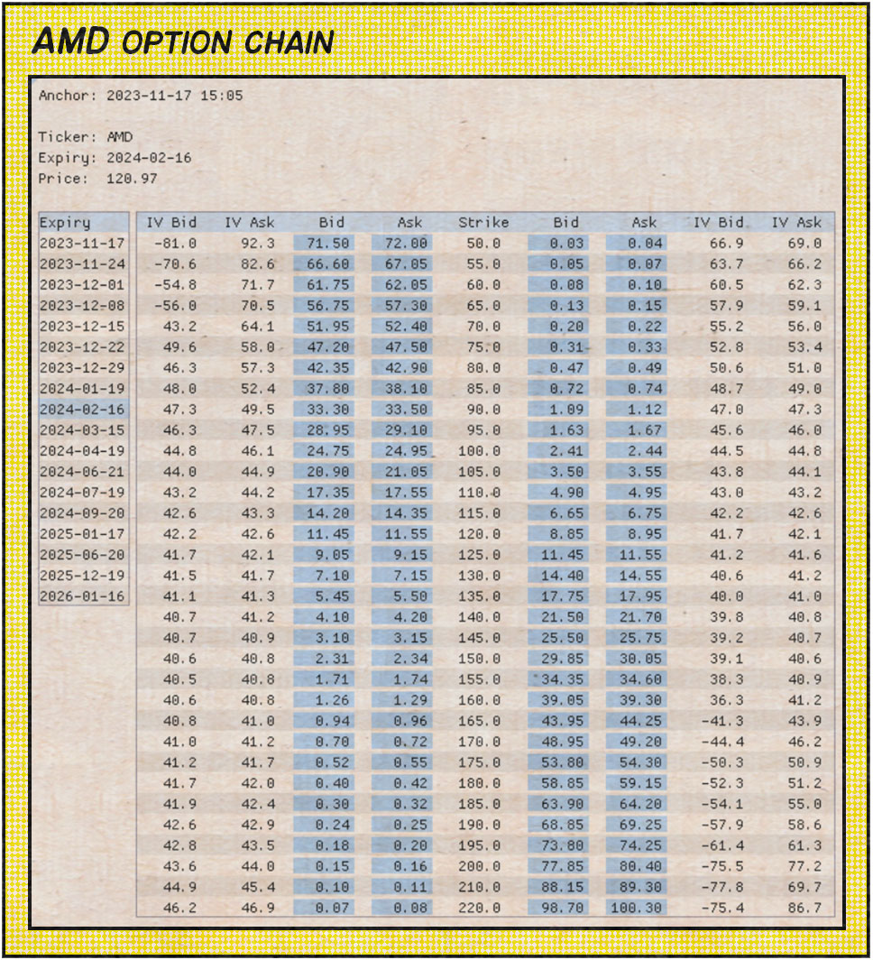
Calibration. For now we solve a pricing problem only, that is to find an option price given implied volatility and option parameters, like strike, expiry, etc. In practice, the implied volatility is unknown and should be determined given the option price from the exchange. This is known as calibration and is the inverse problem to pricing, which we’ll focus on in another post.
For example, below is a chain of option prices and already calibrated implied volatilities for AMD as of 2023-11-17 15:05:
Pricing Equation
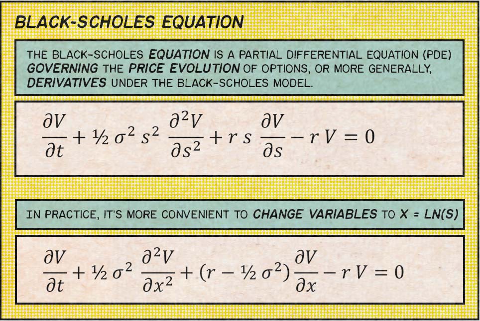
American option’s price is defined as a solution of the Black-Scholes equation. In fact, it’s the same equation that results into a famous Black-Scholes formula for European option. However, for American option we should impose an extra condition to account for the early exercise, which we discuss down below. It’s this early-exercise condition that makes the original equation so difficult that we have no option, but to solve it numerically.
The Black-Scholes equation is just a particular example of the pricing differential equation. In general, we can define similar differential equations for various types and flavours of options and other derivatives, which can be treated with the same method. This versatility is what makes the finite-difference so popular among quants and widely used in financial institutions.
The pricing equation is usually derived using Delta Hedging argument, which is an intuitive and powerful approach to derive pricing equations, not only for vanilla options, but for exotic multi-asset derivatives as well.
In practice, it’s more convenient to change variables to x = ln(s) which leads to the following
equation:
Numerical Solution
The Black-Scholes equation belongs to the family of diffusion equations, which in general case have no closed-form solution. Fortunately it’s one of the easiest differential equations to solve numerically, which apart from the Finite-Difference, are usually treated with Monte-Carlo or Fourier transformation methods.
The Solution. Let’s be more specific about the solution we are looking for. Our goal is to find
the option price function V(t,s) at a fixed time t=0 (today) for arbitrary spot price s.
Here
tis time from today;sis the spot price of the option’s underlying asset. Although, it’s more convenient to work withx = ln(s)instead.
Let’s continue with concrete steps of the finite-difference method:
1) Finite Grid. We define a rectangular grid on the domain of independent variables (t,s)
which take
t[i] = t[i-1] + dt[i]fori=0..N-1x[j] = x[j-1] + dx[j]forj=0..M-1.
This naturally leads to the following C++ definitions:
1u32 xDim = 512;
2u32 tDim = 1024;
3
4std::vector<f64> x(xDim);
5std::vector<f64> t(tDim);
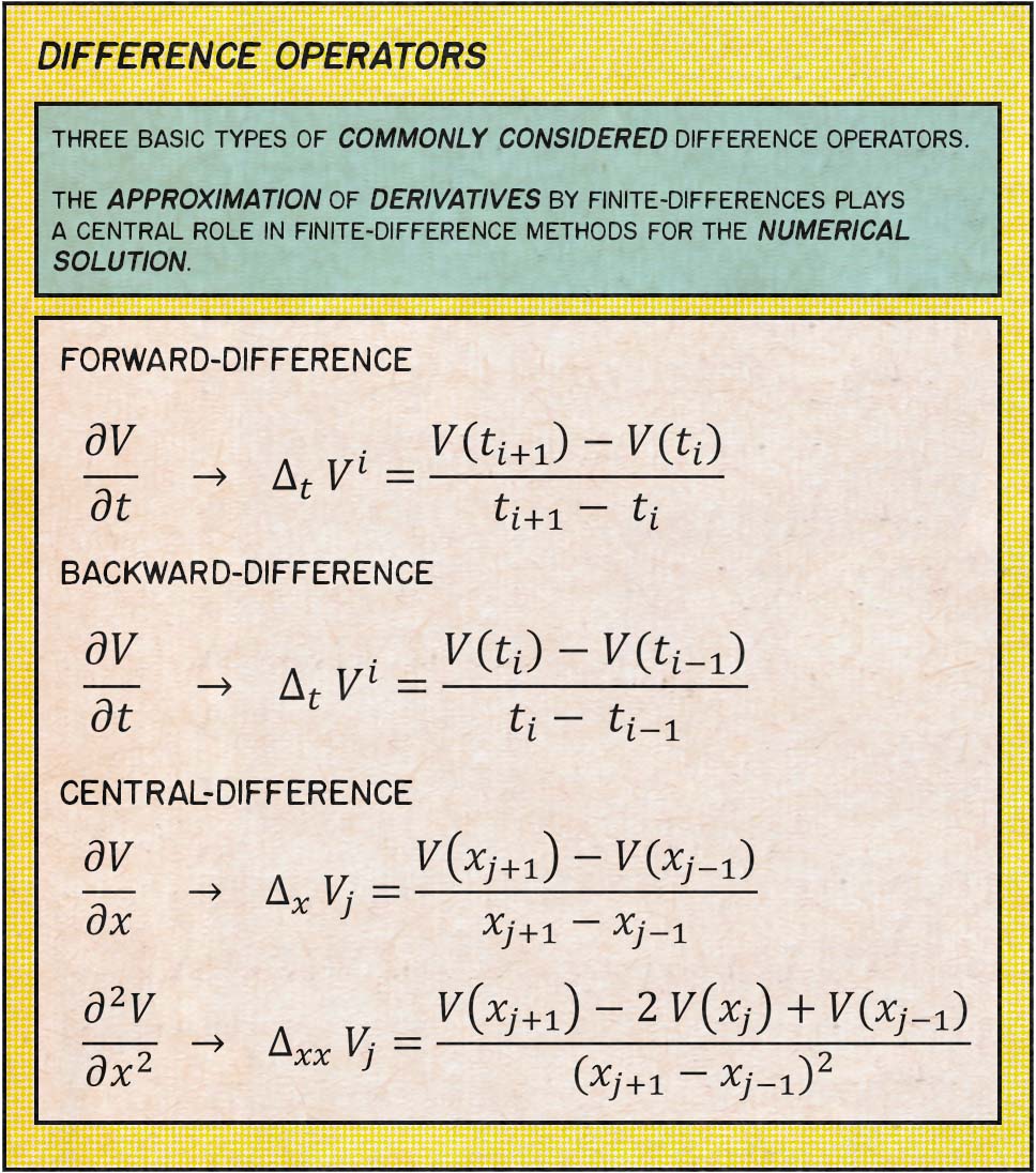
2) Difference Operators are used
to approximate continuous derivatives in the original pricing equation. They are defined on the
(t,x) grid as:
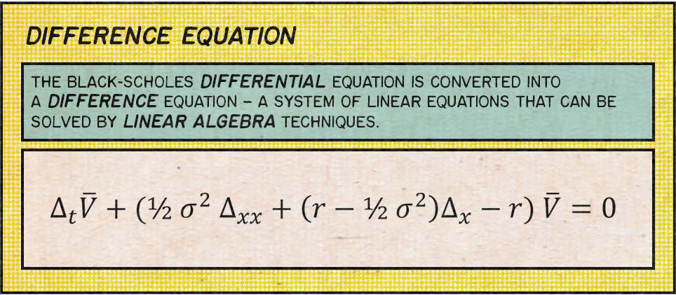
3) Finite-Difference Equation, a discrete version of the Black-Scholes equation, is derived from the pricing equation by replacing continuous derivatives with difference operators defined in Step 2.
It’s convenient to introduce the A operator, which contains difference operators over the x-axis only.
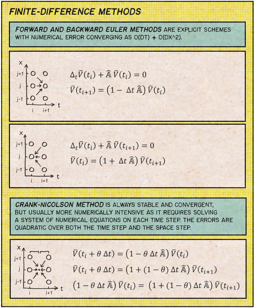
4) Solution Scheme. The above equation isn’t completely defined yet, as we can expand \delta_t operator in several ways. (\delta_x and \delta_xx operators are generally chosen according to the central difference definition.)
\delta_t operator might be chosen as Forward or Backward difference, which lead to the explicit scheme solution. In this case, the numerical error is O(dt) + O(dx^2), which is not the best we can achieve.
Crank-Nicolson scheme, an implicit scheme, is a better alternative to the explicit scheme. It’s slightly more complicated, since requires to solve a liner system of equations, however the numerical error is O(dt^2) + O(dx^2), which is much better than for the explicit schemes.
You can think of the Crank-Nicolson scheme as a continuos mix of forward and backward schemes tuned by \theta parameter, so that
\theta = 1is Euler forward scheme\theta = 0is Euler backward\theta = 1/2is Crank-Nicolson scheme
5) Backward Evolution. I guess at this point it’s clear what our next step should be. All we
need is to solve a tridiagonal linear system in order to find V(t_i) from V(t_i+1) as is
prescribed by the Crank-Nicolson method above. The initial value is given by the option price at
maturity V(t=T), which is equal to the payoff or intrinsic value for a given strike k, in
other words
max(s-k, 0)for calls,max(k-s, 0)for puts.
Thomas algorithm is a simplified form of Gaussian elimination that is used to solve tridiagonal systems of linear equations. For such systems, the solution can be obtained in O(n) operations instead of O(n^3) required by Gaussian elimination, which makes this step relatively fast.
C++ implementation of the Thomas solver is compact and widely available, for example, see Numerical Recipes. I list it below for completeness:
 1Error
 2solveTridiagonal(
 3    const int xDim,
 4    const f64* al, const f64* a, const f64* au,    /// LHS
 5    const f64* y,                                  /// RHS
 6    f64* x)                                        /// Solution
 7{
 8    if (a[0] == 0)
 9        return "solveTridiagonal: Error 1";
10    if (xDim <= 2)
11        return "solveTridiagonal: Error 2";
12
13    std::vector<f64> gam(xDim);
14
15    f64 bet;
16    x[0] = y[0] / (bet = a[0]);
17    for (auto j = 1; j < xDim; j++) {
18        gam[j] = au[j - 1] / bet;
19        bet = a[j] - al[j] * gam[j];
20
21        if (bet == 0)
22            return "solveTridiagonal: Error 3";
23
24        x[j] = (y[j] - al[j] * x[j - 1]) / bet;
25        if (x[j] < 0)
26            continue;
27    };
28
29    for (auto j = xDim - 2; j >= 0; --j) {
30        x[j] -= gam[j + 1] * x[j + 1];
31    }
32
33    return "";
34};
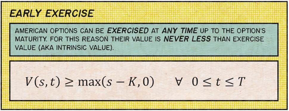
6) Early Exercise. For American options we should taken into account the right to exercise before maturity. As already mention, this particular feature make the Black-Scholes equation more complicated with no closed-form solution.
I account for this at every backward evolution step like this:
1for (auto xi = 0; xi < xDim; ++xi) {
2    v[xi] = std::max(v[xi], vInit[xi]);
3}
Boundary Conditions
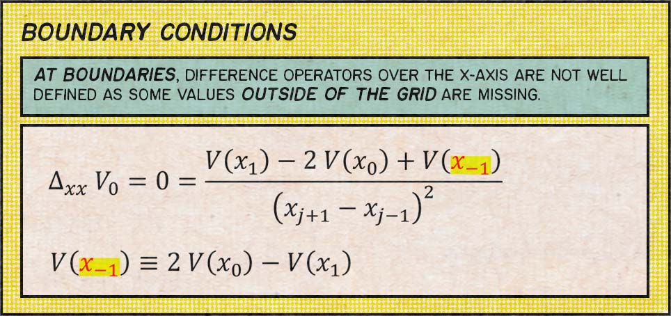
You probably noticed that our definition of the difference operators on the grid is incomplete. Namely, the x-axis difference is not well defined at boundaries of the grid.
At boundaries, difference operators over the x-axis are not well defined as some values outside of the grid are missing. For example,
V'(x_0) = (V(x_1) - V(x_-1)) / (x_1 - x_-1)
however x_-1 and V(x_-1) are not defined.
We overcome this by taking into account the asymptotic behavior of the price function V(t,s) at
boundaries of s, when s -> 0 and s -> +oo.
We know that delta is constant at boundaries, either 0 or 1, depending on the parity (PUT or
CALL). However, more universal relation is that gamma = 0 at boundaries. This gives the following
relation:
Finite-Difference Grid
Finally, it’s time to discuss how grid points are distributed over x- and t-axes. So far we just
said that there are N and M points along each axis, but said nothing about the limits and
distribution of those points. In other words, what are the values x[0] / x[M-1] and gaps dt[i] = t[i+1] - t[i] and dx[i] = x[i+1] - x[i] ?
The t-Axis is divided uniformly with a step dt = T / N between points. It doesn’t seem to use some non-uniform step here, at least not something I observed in practice.
The x-Axis is divided in a more tricky way. …
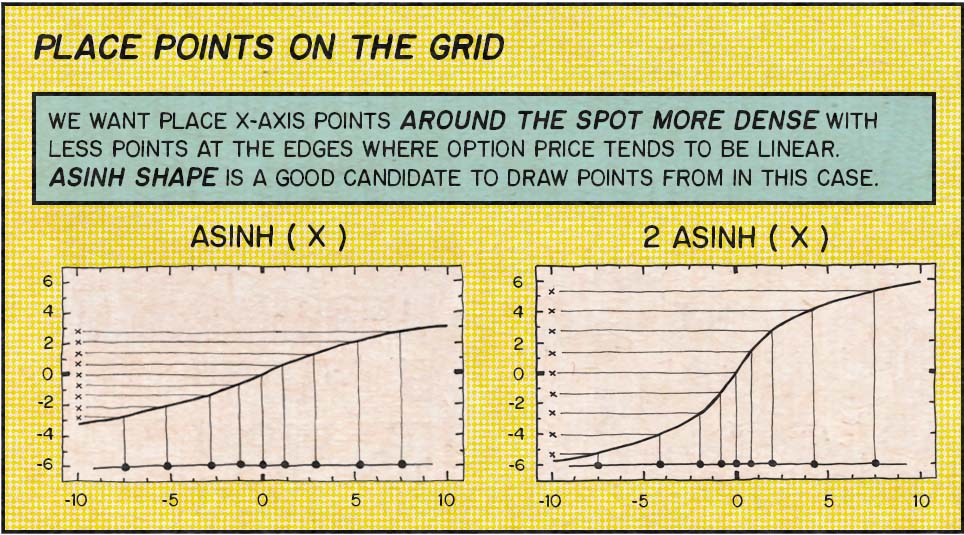
 1/// Init X-Grid
 2
 3const f64 density = 0.1;
 4const f64 scale = 10;
 5
 6const f64 xMid = log(s);
 7const f64 xMin = xMid - scale * z * sqrt(t);
 8const f64 xMax = xMid + scale * z * sqrt(t);
 9
10const f64 yMin = std::asinh((xMin - xMid) / density);
11const f64 yMax = std::asinh((xMax - xMid) / density);
12
13const f64 dy = 1. / (xDim - 1);
14for (auto j = 0; j < xDim; j++) {
15    const f64 y = j * dy;
16    xGrid(j) = xMid + density * std::sinh(yMin * (1.0 - y) + yMax * y);
17}
18
19/// Inspired by https://github.com/lballabio/QuantLib files:
20///   - fdmblackscholesmesher.cpp
21///   - fdblackscholesvanillaengine.cpp
Conclusion
In this post I elaborated on some key parts of my C++ implementation of the finite-difference pricer for American options, which is available in gituliar/kwinto-cuda repo on GitHub. The method itself can be applied to a wide range of problems in finance which makes it so popular among quants.
Also, take a look at my previous post Pricing Derivatives on a Budget, where I discussed performance of this finite-difference algorithm for pricing American options on CPU vs GPU.
References
- Lectures on Finite-Difference Methods by Andreasen and Huge
- Numerical Recipes in C++