

After five years working as a quant, I can tell that the wast majority of derivative pricing in the financial industry is done on CPU. This is easily explained by two facts: (1) no GPU was available when banks started developing their pricing analytics in 90’s; and (2) banking is a conservative sector, slow to upgrade its technical stack.
American Options. In this post, I benchmark pricing of American Options on GPU. Since no analytical formula exist to price American options (similar to the Black-Scholes formula for European options), people in banks use numerical methods to solve this sort of problems. Such methods are computationally greedy and, in practice, require a lot of hardware to risk-manage trading books with thousands of positions.
Finite Difference. For the benchmark, I use my own implementations of the finite-difference method for CPU and GPU. When it comes to pricing derivatives, there are two methods, widely-adopted by the industry, that are capable to solve a wide range of pricing problems. The first one is the famous Monte-Carlo method. Another one is the Finite-Difference method, which we will focus on in this post today.
Note, a much faster method to price American Options was recently developed by Andersen et al. (details below). This method has some constraints (like time-independent coefficients or log-normal underlying process) and is not a complete replacement for the finite-difference.
Source Code. The code is written in C++ / CUDA and is available on Github: https://github.com/gituliar/kwinto-cuda. It’s compatible with Linux and Windows, but requires Nvidia GPU.
The finite-difference algorithm itself is not very complicated, however deserves a dedicated post to be fully explained, as there are some nuances here and there. Hopefully, I’ll find some time to cover this topic later.
Main focus of the benchmarking is on the following:
- How much faster is GPU vs CPU? Speed is a convenient metric to compare performance, as faster usually means better (given all other factors equal).
- How much cheaper is GPU vs CPU? Budget is always important when making decisions. Speed matters because fast code means less CPU time, but there are other essential factors worth discussing that impact your budget.
Benchmark
My approach is to price american options in batches. This is usually how things are run in banks, when risk-managing trading books. Every batch contains from 256 to 16'384 american options, which are priced in parallel utilizing all cores on CPU or GPU.
The total pool of 378'000 options for the benchmark is constructed by permuting all combinations of the following parameters (with options cheaper than 0.5 rejected). Reference prices are calculated with portfolio.py in QuantLib, using the Spanderen implementation of a high-performance Andersen-Lake-Offengenden algorithm for pricing american options.
| Parameter | Range |
|---|---|
| Parity | PUT |
| Strike | 100 |
| Spot | 25, 50, 80, 90, 100, 110, 120, 150, 175, 200 |
| Maturity | 1/12, 0.25, 0.5, 0.75, 1.0, 1.25, 1.5, 1.75, 2.0 |
| Volatility | 0.1, 0.2, 0.3, 0.4, 0.5, 0.6, 0.7, 0.8, 0.9, 1.0, 1.1, 1.2, 1.3, 1.4, 1.5 |
| Interest rate | 1%, 2%, 3%, 4%, 5%, 6%, 7%, 8%, 9%, 10% |
| Dividend rate | 0%, 2%, 4%, 6%, 8%, 10%, 12% |
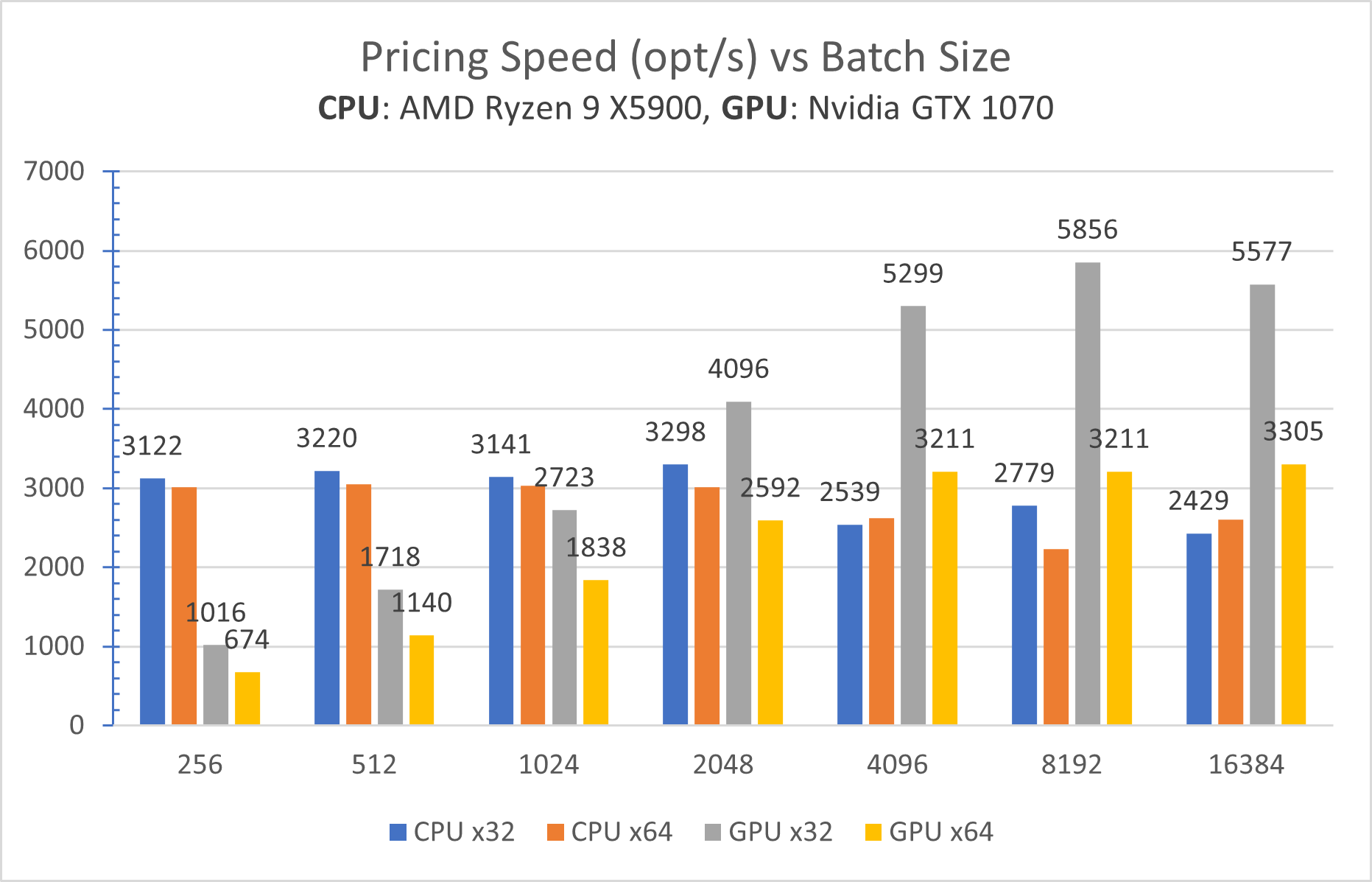
Results. A plot below depicts the main results. Each bin shows how many options are priced per second (higher is better):
US Options Market. To get some idea about how these results are useful in practice, let’s have a look at a size of the US options market. The data from OPRA tells that there are:
- 5'800 stocks
- 680'000 options (with 5%-95% delta)
In other words, as per the benchmark, it takes 2 min to price an entire US Options Market on a $100 GPU. It should take 10x longer for calibration, which is a more challenging task.
Few things to keep in mind for the results above:
-
GPU is 2x faster in a single-precision mode (gray bin) vs double-precision (yellow bin). Meantime, CPU performs more or less the same in both modes (blue and orange bins).
This is a clear sign that the GPU is limited by data throughput. With its 1'920 cores, the GPU processes data faster than loads it from the GPU memory.
-
GPU is 4 years older, which is a big gap for hardware. Nevertheless, the oldish GPU is still faster than the modern CPU.
- Nvidia GTX 1070, 16nm – released in 2016.
- AMD Ryzen 9 X5900, 7nm – released in 2020.
Budget
In the production environment, faster is almost always means cheaper. Speed is not the only factor that affects operational costs. Let’s take a look at other factors that appeal in favor of GPU:
Cheap to scale. To run an extra CPU it requires a motherboard, RAM, HDD – a whole new machine, which quickly becomes expensive to scale.
An extra GPU, however, requires only a PCI-E slot. Some motherboards offer a dozen PCI-E ports, like ASRock Q270 Pro BTC+, which is especially popular among crypto miners. Such a motherboard can handle 17 GPUs on a single machine. In addition, there is no need to setup a network, manage software on various machines, and hire an army of devops to automate all that.
This gives extra 3-5x cost reduction in favor of GPU.
Cheap to upgrade. PCI-E standard is backward compatible, so that new GPU cards are still run on old machines. Below is the same benchmark run on a much older machine with dual Xeon X5675 from 2011:
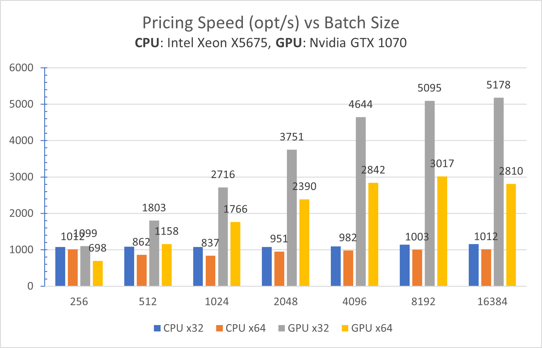
What immediately catches the eye is that Ryzen 9 outperforms the dual-Xeon machine (both have equal number of physical cores, btw). This is not a surprise, given a 10-year technological gap.
Surprising is that a newer GPU performs equally well on a much older machine. In practice, this means that at some point in the future when GPU cards deserve an upgrade there is no need to upgrade other components, like CPU, motherboard, etc.
Summary
The Finite-Difference method is a universal and powerful method, heavily used in the financial industry. However, what is the benefit of running it on GPU ?
Final verdict. My benchmark shows that:
- GPU is 2x faster
- GPU is 3x-5x cheaper
This combined gives 10x factor in favor of GPU as a platform for pricing derivatives.